Page 25 - Fister jr., Iztok, Andrej Brodnik, Matjaž Krnc and Iztok Fister (eds.). StuCoSReC. Proceedings of the 2019 6th Student Computer Science Research Conference. Koper: University of Primorska Press, 2019
P. 25
er deleting the chosen edges, we determined the dis- When we used the graph of Germany, the results were dif-
tance matrix on the modified graph. In order to get the ferent. The tendency was the same, but the amount of the
distances, we used the definition of shortest path, and the rise of the solution was much lower. First we located only
Ford-Fulkerson algorithm. one facility. By deleting 10% of the edges and locating one
facility the cost increased by 10% (minimum 1% and maxi-
4. RESULTS AND ANALYSIS mum 23%). By deleting more edges, the solution increased
slightly, but not as much as with the Italian graph. When
The algorithm was tested on two data files, modeling the we deleted 40% of the edges, the cost increased with 84%
largest cities and roads of Italy and Germany. In order to on average (minimum 57%, maximum 124%). As with the
have a better view on the results, we draw the graphs using previous graph, we repeated the test by locating two and
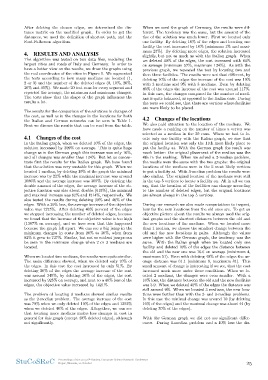
the real coordinates of the cities in Figure 1. We segmented then three facilities. The results were not that different, by
the tests according to how many medians are located (1, deleting 10% of the edges the increase of the cost was 10%
2 or 3) and the number of the deleted edges (0, 10%, 20%, with 2 medians and 9% with 3 medians. Even by deleting
30% and 40%). We made 20 test runs for every segment and 40% of the edges the increase of the cost was around 117%.
reported the average, the minimum and maximum changes. In this case, the changes compared for the number of medi-
The tests show that the shape of the graph influences the ans is quite balanced, as opposed to the Italian case. During
results a lot. the tests we could see, that there are vertices where facilities
are more likely to be placed.
The results for the comparison of the solutions in changes of
the cost, as well as in the changes in the locations for both 4.2 Changes of the locations
the Italian and German networks can be seen in Table 1.
Next we discuss the results that can be read from the table. We also paid attention to the location of the medians. We
have made a ranking on the number of times a vertex was
4.1 Changes of the cost selected as a median in the 20 runs. When we had to lo-
cate only one facility with the Italian graph, we saw that
In the Italian graph, when we deleted 10% of the edges, the the original location was only the 11th most likely place to
solution increased by 309% on average. This is quite huge put the facility at. With the German graph the result was
change as in the German graph this increase was only 10%, much better: the original placement of the median was the
and all changes was smaller than 134%. But let us concen- 4th in the ranking. When we solved a 2-median problem,
trate first the results for the Italian graph. We have found the results were the same with the two graphs: the original
that the solution was very unstable for this graph. When we locations of the medians were in the 5 most likely vertices
located 1 median, by deleting 10% of the graph the minimal to put a facility at. With 3-median problem the results were
increase was by 22% while the maximal increase was around also similar. The original location of the medians were still
1086% and the average increase was 309%. By deleting the in the top 5 vertices to locate a facility on. All in all we can
double amount of the edges, the average increase of the ob- say, that the location of the facilities can change according
jective function was also about double (615%), the minimal to the number of deleted edges, but the original locations
and maximal increase was 82% and 1314%, respectively. We are almost always in the top 5 vertices.
also tested the results during deleting 30% and 40% of the
edges. With a 30% loss, the average increase of the objective During our research we also made computations to inspect,
value was 1275%. After deleting 40% percent of the edges how far the new locations from the old ones are. To get an
we stopped increasing the number of deleted edges, because objective picture about the results we always used the orig-
we found that the increase of the objective value is too high inal graphs and the shortest distances between the old and
(1387% on average), and we have seen that this happened the new locations of the medians. When we located more
because the graph fell apart. We can see a big jump in the than 1 median, we choose the smallest change between the
minimum changes in costs from 20% to 30%, when from old and the new locations in pairs. Although the values
82% it grew to 737%. Similar, but not so evident jumps can were higher with the German graph, the tendency was the
be seen in the minimum change when 2 or 3 medians are same. With the Italian graph when we located only one
located. facility and deleted 10% of the edges the distance between
the old and the new one was 16.6 on average (minimum 4,
When we located two medians, the results were quite similar. maximum 51). Even with deleting 40% of the edges the av-
The main difference showed, when we deleted only 10% of erage distance was 61.1 (minimum 8, maximum 81). This
the edges. In this case the cost increased by only 51%. By small amount of change is interesting if we see, that the cost
deleting 20% of the edges the average increase of the cost increased much more under these conditions. When we lo-
was around 345%, by deleting 30% of the edges, the cost cated 2 medians, the changes were even smaller. With a
increased by 925% on average, and next to a 40% loss of the 10% loss, the distance between the old and the new facilities
edges, the objective value increased by 1421%. was 3.9. When we deleted 40% of the edges the distance was
still around 9%. When we located 3 medians, the new loca-
The problem of locating 3 medians showed similar results tions were farther than with the 2- and 3-median problems.
as the 2-median problem. The average increase of the cost In this case the minimal change was around 10 (by deleting
was 79% when we only deleted 10% of the edges and 1352% 10% of the edges) and the maximal change was about 44 (by
when we deleted 40% of the edges. Altogether, we can see deleting 30% of the edges).
that locating more medians makes less changes in cost in
general for this graph (except 40% deleted edges), although With the German graph we did not see significant differ-
not significantly. ences. During 1-median problem and a 10% loss the dis-
StuCoSReC Proceedings of the 2019 6th Student Computer Science Research Conference 25
Koper, Slovenia, 10 October
tance matrix on the modified graph. In order to get the ferent. The tendency was the same, but the amount of the
distances, we used the definition of shortest path, and the rise of the solution was much lower. First we located only
Ford-Fulkerson algorithm. one facility. By deleting 10% of the edges and locating one
facility the cost increased by 10% (minimum 1% and maxi-
4. RESULTS AND ANALYSIS mum 23%). By deleting more edges, the solution increased
slightly, but not as much as with the Italian graph. When
The algorithm was tested on two data files, modeling the we deleted 40% of the edges, the cost increased with 84%
largest cities and roads of Italy and Germany. In order to on average (minimum 57%, maximum 124%). As with the
have a better view on the results, we draw the graphs using previous graph, we repeated the test by locating two and
the real coordinates of the cities in Figure 1. We segmented then three facilities. The results were not that different, by
the tests according to how many medians are located (1, deleting 10% of the edges the increase of the cost was 10%
2 or 3) and the number of the deleted edges (0, 10%, 20%, with 2 medians and 9% with 3 medians. Even by deleting
30% and 40%). We made 20 test runs for every segment and 40% of the edges the increase of the cost was around 117%.
reported the average, the minimum and maximum changes. In this case, the changes compared for the number of medi-
The tests show that the shape of the graph influences the ans is quite balanced, as opposed to the Italian case. During
results a lot. the tests we could see, that there are vertices where facilities
are more likely to be placed.
The results for the comparison of the solutions in changes of
the cost, as well as in the changes in the locations for both 4.2 Changes of the locations
the Italian and German networks can be seen in Table 1.
Next we discuss the results that can be read from the table. We also paid attention to the location of the medians. We
have made a ranking on the number of times a vertex was
4.1 Changes of the cost selected as a median in the 20 runs. When we had to lo-
cate only one facility with the Italian graph, we saw that
In the Italian graph, when we deleted 10% of the edges, the the original location was only the 11th most likely place to
solution increased by 309% on average. This is quite huge put the facility at. With the German graph the result was
change as in the German graph this increase was only 10%, much better: the original placement of the median was the
and all changes was smaller than 134%. But let us concen- 4th in the ranking. When we solved a 2-median problem,
trate first the results for the Italian graph. We have found the results were the same with the two graphs: the original
that the solution was very unstable for this graph. When we locations of the medians were in the 5 most likely vertices
located 1 median, by deleting 10% of the graph the minimal to put a facility at. With 3-median problem the results were
increase was by 22% while the maximal increase was around also similar. The original location of the medians were still
1086% and the average increase was 309%. By deleting the in the top 5 vertices to locate a facility on. All in all we can
double amount of the edges, the average increase of the ob- say, that the location of the facilities can change according
jective function was also about double (615%), the minimal to the number of deleted edges, but the original locations
and maximal increase was 82% and 1314%, respectively. We are almost always in the top 5 vertices.
also tested the results during deleting 30% and 40% of the
edges. With a 30% loss, the average increase of the objective During our research we also made computations to inspect,
value was 1275%. After deleting 40% percent of the edges how far the new locations from the old ones are. To get an
we stopped increasing the number of deleted edges, because objective picture about the results we always used the orig-
we found that the increase of the objective value is too high inal graphs and the shortest distances between the old and
(1387% on average), and we have seen that this happened the new locations of the medians. When we located more
because the graph fell apart. We can see a big jump in the than 1 median, we choose the smallest change between the
minimum changes in costs from 20% to 30%, when from old and the new locations in pairs. Although the values
82% it grew to 737%. Similar, but not so evident jumps can were higher with the German graph, the tendency was the
be seen in the minimum change when 2 or 3 medians are same. With the Italian graph when we located only one
located. facility and deleted 10% of the edges the distance between
the old and the new one was 16.6 on average (minimum 4,
When we located two medians, the results were quite similar. maximum 51). Even with deleting 40% of the edges the av-
The main difference showed, when we deleted only 10% of erage distance was 61.1 (minimum 8, maximum 81). This
the edges. In this case the cost increased by only 51%. By small amount of change is interesting if we see, that the cost
deleting 20% of the edges the average increase of the cost increased much more under these conditions. When we lo-
was around 345%, by deleting 30% of the edges, the cost cated 2 medians, the changes were even smaller. With a
increased by 925% on average, and next to a 40% loss of the 10% loss, the distance between the old and the new facilities
edges, the objective value increased by 1421%. was 3.9. When we deleted 40% of the edges the distance was
still around 9%. When we located 3 medians, the new loca-
The problem of locating 3 medians showed similar results tions were farther than with the 2- and 3-median problems.
as the 2-median problem. The average increase of the cost In this case the minimal change was around 10 (by deleting
was 79% when we only deleted 10% of the edges and 1352% 10% of the edges) and the maximal change was about 44 (by
when we deleted 40% of the edges. Altogether, we can see deleting 30% of the edges).
that locating more medians makes less changes in cost in
general for this graph (except 40% deleted edges), although With the German graph we did not see significant differ-
not significantly. ences. During 1-median problem and a 10% loss the dis-
StuCoSReC Proceedings of the 2019 6th Student Computer Science Research Conference 25
Koper, Slovenia, 10 October