Page 29 - Fister jr., Iztok, Andrej Brodnik, Matjaž Krnc and Iztok Fister (eds.). StuCoSReC. Proceedings of the 2019 6th Student Computer Science Research Conference. Koper: University of Primorska Press, 2019
P. 29
e are randomly chosen. If the assignment of the current • Swap: The timeslot of a (course, timeslot,room) as-
course is not possible to this node, then another one is cho- signment is swapped with the slot of another assign-
sen and a recursive call is made. If the course is compatible ment.
with the node, and the teacher of the course is also available
at the time-slot in question, then the assignment is saved, • Move: A (course,timeslot,room) assignment is moved
and the next recursive call will feature a new course. The al- to another (timeslot,room) position.
gorithm terminates if all the courses are assigned, or if there
are no more possible nodes to choose from. The process examines all possible neighborhood moves for
a given timetable, and applies the one with the smallest
As the initial solution is built without considering any soft penalty. If the resulting timetable is better than the cur-
constraints, it will have a high penalty. A local search rently stored best one, then it becomes the new best solu-
method is then used to decrease this penalty by also tak- tion, and the neighborhood move that was used to produce
ing the soft constraints of the problem into consideration. this solution is saved to the tabu list of forbidden moves.
The outline of the algorithm can be seen in Algorithm 2.
If a local optimum is found, the algorithm switches to the
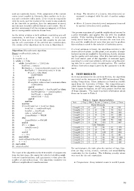
Algorithm 2 Local search algorithm. destructSearch phase. In this phase, a set number of neigh-
borhood moves are applied to the solution, strictly decreas-
Funct localSearch(tt, tabu, n) ing the quality with each step. After this destruction phase,
the local search part of the algorithm is executed again,
1: i := 0 searching for a new local optimum, while also using the exist-
2: bestSol := tt ing tabu list to avoid certain transformations. The number
3: while n > 0 do of these destruction steps is given by the parameter n in the
4: while f oundBetter = TRUE do input.
5: bestCost = cost(tt)
6: for Each a := (course,timeslot,room) in tt do 4. TEST RESULTS
7: for Each b := (timeslot,room) in tt do
8: if (a,b) ∈ tabu then As it was mentioned in the previous Section, the algorithm
9: CONTINUE was tested on the instances of the 2007 International Time-
10: end if tabling Competition. These instances are based on real-life
11: neighbor := tt.swap(a,b) input from the University of Udine. The competition pro-
12: if neighbor violates hard constraints then vided three sets of input: Early, Late and Hidden datasets.
13: CONTINUE Due to space limitations, we will only present the first two
14: end if of these datasets. The most important information about
15: if cost(neighbor) < bestN eighCost then these can be seen in Table 1.
16: bestN eighCost := cost(neighbor)
17: bestN eigh := neighbor Table 1: Input characteristics
18: tabutCand := (b,a)
19: end if Inst. Day Slot Room Course Curr. Unav.
20: end for
21: end for Comp01 Early Datasets 53
22: if bestN eighCost < bestCost then Comp02 513
23: bestCost := cost(bestN eigh) Comp03 5 6 6 30 14 382
24: bestSol := bestN eigh Comp04 396
25: tabu ← tabuCand Comp05 5 5 16 82 70 771
26: f oundBetter := TRUE Comp06 632
27: else Comp07 5 5 16 72 68 667
28: f oundBetter := FALSE
29: end if Comp08 5 5 18 79 57 478
30: if i > x then Comp09 405
31: tabu(0).erase() Comp10 6 6 9 54 139 694
32: i := 0 Comp11 94
33: end if Comp12 5 5 18 108 70 1368
34: i := i+1 Comp13 468
35: end while Comp14 5 5 20 131 77 486
36: destructSearch(bestSol, tabu)
37: n := n-1 Late Datasets
38: end while
39: return bestSol 5 5 18 86 61
The input of the algorithm is the tt timetable of assignments 5 5 18 76 75
from the first stage, the empty list tabu for forbidden neigh-
borhood transformations, and a parameter n that gives the 5 5 18 115 67
number of destruction steps. The algorithm considers two
different neighborhood transformations: 5 9 5 30 13
6 6 11 88 150
5 5 19 82 66
5 5 17 85 60
For each instance, the table gives the number of days, time-
slots per day, rooms, courses, curricula and unavailability
constraints for the teachers. The following penalty values
were used for the soft constraints:
• Compactness: Every isolated course is worth 2 ponts.
StuCoSReC Proceedings of the 2019 6th Student Computer Science Research Conference 29
Koper, Slovenia, 10 October
course is not possible to this node, then another one is cho- signment is swapped with the slot of another assign-
sen and a recursive call is made. If the course is compatible ment.
with the node, and the teacher of the course is also available
at the time-slot in question, then the assignment is saved, • Move: A (course,timeslot,room) assignment is moved
and the next recursive call will feature a new course. The al- to another (timeslot,room) position.
gorithm terminates if all the courses are assigned, or if there
are no more possible nodes to choose from. The process examines all possible neighborhood moves for
a given timetable, and applies the one with the smallest
As the initial solution is built without considering any soft penalty. If the resulting timetable is better than the cur-
constraints, it will have a high penalty. A local search rently stored best one, then it becomes the new best solu-
method is then used to decrease this penalty by also tak- tion, and the neighborhood move that was used to produce
ing the soft constraints of the problem into consideration. this solution is saved to the tabu list of forbidden moves.
The outline of the algorithm can be seen in Algorithm 2.
If a local optimum is found, the algorithm switches to the
Algorithm 2 Local search algorithm. destructSearch phase. In this phase, a set number of neigh-
borhood moves are applied to the solution, strictly decreas-
Funct localSearch(tt, tabu, n) ing the quality with each step. After this destruction phase,
the local search part of the algorithm is executed again,
1: i := 0 searching for a new local optimum, while also using the exist-
2: bestSol := tt ing tabu list to avoid certain transformations. The number
3: while n > 0 do of these destruction steps is given by the parameter n in the
4: while f oundBetter = TRUE do input.
5: bestCost = cost(tt)
6: for Each a := (course,timeslot,room) in tt do 4. TEST RESULTS
7: for Each b := (timeslot,room) in tt do
8: if (a,b) ∈ tabu then As it was mentioned in the previous Section, the algorithm
9: CONTINUE was tested on the instances of the 2007 International Time-
10: end if tabling Competition. These instances are based on real-life
11: neighbor := tt.swap(a,b) input from the University of Udine. The competition pro-
12: if neighbor violates hard constraints then vided three sets of input: Early, Late and Hidden datasets.
13: CONTINUE Due to space limitations, we will only present the first two
14: end if of these datasets. The most important information about
15: if cost(neighbor) < bestN eighCost then these can be seen in Table 1.
16: bestN eighCost := cost(neighbor)
17: bestN eigh := neighbor Table 1: Input characteristics
18: tabutCand := (b,a)
19: end if Inst. Day Slot Room Course Curr. Unav.
20: end for
21: end for Comp01 Early Datasets 53
22: if bestN eighCost < bestCost then Comp02 513
23: bestCost := cost(bestN eigh) Comp03 5 6 6 30 14 382
24: bestSol := bestN eigh Comp04 396
25: tabu ← tabuCand Comp05 5 5 16 82 70 771
26: f oundBetter := TRUE Comp06 632
27: else Comp07 5 5 16 72 68 667
28: f oundBetter := FALSE
29: end if Comp08 5 5 18 79 57 478
30: if i > x then Comp09 405
31: tabu(0).erase() Comp10 6 6 9 54 139 694
32: i := 0 Comp11 94
33: end if Comp12 5 5 18 108 70 1368
34: i := i+1 Comp13 468
35: end while Comp14 5 5 20 131 77 486
36: destructSearch(bestSol, tabu)
37: n := n-1 Late Datasets
38: end while
39: return bestSol 5 5 18 86 61
The input of the algorithm is the tt timetable of assignments 5 5 18 76 75
from the first stage, the empty list tabu for forbidden neigh-
borhood transformations, and a parameter n that gives the 5 5 18 115 67
number of destruction steps. The algorithm considers two
different neighborhood transformations: 5 9 5 30 13
6 6 11 88 150
5 5 19 82 66
5 5 17 85 60
For each instance, the table gives the number of days, time-
slots per day, rooms, courses, curricula and unavailability
constraints for the teachers. The following penalty values
were used for the soft constraints:
• Compactness: Every isolated course is worth 2 ponts.
StuCoSReC Proceedings of the 2019 6th Student Computer Science Research Conference 29
Koper, Slovenia, 10 October