Page 59 - Fister jr., Iztok, Andrej Brodnik, Matjaž Krnc and Iztok Fister (eds.). StuCoSReC. Proceedings of the 2019 6th Student Computer Science Research Conference. Koper: University of Primorska Press, 2019
P. 59
nge is not applied to the backward pass. All these procedures Once we had the data in the required type and form, we started
help to make the model generalizable. building the RNN model. We used again as a input data values from
the electrodes (Af3, T7, P7, T8, Af4).
When we had finished defining the model, we still had to compile
the model with a function that would define a loss (optimizer) that For which we defined the model type as sequential. We added a
would be able to update the weights according to the result and a SimpleRNN level with 32 dimensions and two Dense levels to
function that would return us the result, with what precision in the model, the first with 8 dimensions and the output with one. For
percent, the model predicted the result with given parameters simplicity, we used activation function Relu.
(weights and bias).
Finally, when we built the model, we further defined the
model.compile(loss="binary_crossentropy", optimization function as RmsProp which is designed for RNN
optimizer="adam", models and the loss function as the average squared error.
metrics=['accuracy'])
model = Sequential()
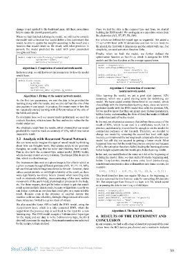
Algorithm 2. Compilation of neural network model. model.add(SimpleRNN(units=32,
In the next step, we still had to set the parameters for how the model input_shape=(1, 5),
would learn. activation="relu"))
model.add(Dense(1))
model.fit(x_train, model.compile(loss='mse',
y_train, optimizer='rmsprop',
batch_size=124, metrics=['accuracy'])
epochs=1000,
validation_data=(x_test, y_test)) Algorithm 6. Construction of recurrent
neural network model.
Algorithm 3. Fitting of the neural network model.
After learning the model, we got a good start (approx. 62%
As the first two parameters, we sent the data to be provided for accuracy), which was a good starting point for optimizing our
learning along with the results, and we also defined the size of the model. We have added another Dense level to our model, which
data packets in one epoch. In practice, this meant more or less that should help with the intermediate learning steps, since we want to
we repeatedly started learning with different values of the size of get better results with the RNN model than with the previous NN,
the batch and epoch. but we need to know that there are many more factors (parameters,
hidden levels, understanding the flow of data) that make it difficult
To determine how well our neural model performed, we used the to understand and refine the model.
evaluate function, which returns the loss and metric values for the
model under test. In the end, we obtained an accuracy that defines the accuracy of the
result of 80%, which in our case is a satisfactory result, but in
We obtained a result from the results, which showed that our model practice, unfortunately, it would not be enough to use the model for
predicted the result to reach an accuracy of 55%, which was not an commercial purposes or for research. Therefore, we decided to
impressive result. change our model by removing the second last level with eight
neurons, as it improved the learning result compared to the previous
3.2 Analysis with Recurrent Neural Network model but still did not succeed in getting a better result. What
happened here was that the model became too complex and because
We can more easily imagine this type of neural model by thinking of this, the activation functions failed, leading the learning phase to
about how our thoughts work, they always relate to our previous better weight adjustments that would give better learning results.
thoughts, we could say that we never start thinking from scratch.
This is also how the recurrent-type neural model (RNN) works, In the end, our model looked the same as it did at the beginning of
which does not restart at every iteration. Traditional NNs do not do defining the model. Here, we then started from the beginning and,
this, which is a disadvantage. before SimpleRNN, inserted a new entry level (Embeding),
which transforms positive data with numbers into dense vectors, for
Our brainwaves data read on a given image is like a list in which at example:
a given moment, through different positions (Af3, T7, P7, T8, Af4),
we can find out which image was shown to the user. However, these [[4], [20]] → [[0.25, 0.1], [0.6, - 0.2]]
values cannot provide us with high reliability of the result, as there
were significantly too many factors present when recording data This level therefore does not require 3D data at the beginning, so
such as electrode reliability, deconcentrating of the user, sudden we also removed the line from our code for converting 2D data into
movements of the user's head, physiological processes in the body, 3D. The output type from Embeding layer is in 3D, which suited
etc. For these reasons, it might be better to want to get that search us in passing the data to our SimpleRNN layer.
result across multiple data records, because within those records we
can define a pattern in our data that could give us a more reliable model = Sequential()
result. Because even in the presence of external factors that model.add(Embedding(10000, 124))
interfere with our data reliability, through a large amount of records model.add(SimpleRNN(32))
these values are limited to a given stock of values. model.add(Dense(1, activation='sigmoid'))
model.compile(loss = "mse",
We also used the Keras API to build the RNN model, using the
SimpleRNN layer, which is a fully connected RNN, where the optimizer = "rmsprop",
output from the previous step is sent back to the input for a new metrics=['accuracy'])
learning step. The RNN model accepts a 3-dimensional input type
for the input, and our data is in the 2-dimensional type, the third Algorithm 8. The final RNN model.
data will represent the step here. Data transformation was achieved
by the numpy.reshape method. 4. RESULTS OF THE EXPERIMENT AND
CONCLUSION
In our scenario, we had a collection of data that represented the read
values from the BCI device per channel and a marker to indicate
StuCoSReC Proceedings of the 2019 6th Student Computer Science Research Conference 59
Koper, Slovenia, 10 October
help to make the model generalizable. building the RNN model. We used again as a input data values from
the electrodes (Af3, T7, P7, T8, Af4).
When we had finished defining the model, we still had to compile
the model with a function that would define a loss (optimizer) that For which we defined the model type as sequential. We added a
would be able to update the weights according to the result and a SimpleRNN level with 32 dimensions and two Dense levels to
function that would return us the result, with what precision in the model, the first with 8 dimensions and the output with one. For
percent, the model predicted the result with given parameters simplicity, we used activation function Relu.
(weights and bias).
Finally, when we built the model, we further defined the
model.compile(loss="binary_crossentropy", optimization function as RmsProp which is designed for RNN
optimizer="adam", models and the loss function as the average squared error.
metrics=['accuracy'])
model = Sequential()
Algorithm 2. Compilation of neural network model. model.add(SimpleRNN(units=32,
In the next step, we still had to set the parameters for how the model input_shape=(1, 5),
would learn. activation="relu"))
model.add(Dense(1))
model.fit(x_train, model.compile(loss='mse',
y_train, optimizer='rmsprop',
batch_size=124, metrics=['accuracy'])
epochs=1000,
validation_data=(x_test, y_test)) Algorithm 6. Construction of recurrent
neural network model.
Algorithm 3. Fitting of the neural network model.
After learning the model, we got a good start (approx. 62%
As the first two parameters, we sent the data to be provided for accuracy), which was a good starting point for optimizing our
learning along with the results, and we also defined the size of the model. We have added another Dense level to our model, which
data packets in one epoch. In practice, this meant more or less that should help with the intermediate learning steps, since we want to
we repeatedly started learning with different values of the size of get better results with the RNN model than with the previous NN,
the batch and epoch. but we need to know that there are many more factors (parameters,
hidden levels, understanding the flow of data) that make it difficult
To determine how well our neural model performed, we used the to understand and refine the model.
evaluate function, which returns the loss and metric values for the
model under test. In the end, we obtained an accuracy that defines the accuracy of the
result of 80%, which in our case is a satisfactory result, but in
We obtained a result from the results, which showed that our model practice, unfortunately, it would not be enough to use the model for
predicted the result to reach an accuracy of 55%, which was not an commercial purposes or for research. Therefore, we decided to
impressive result. change our model by removing the second last level with eight
neurons, as it improved the learning result compared to the previous
3.2 Analysis with Recurrent Neural Network model but still did not succeed in getting a better result. What
happened here was that the model became too complex and because
We can more easily imagine this type of neural model by thinking of this, the activation functions failed, leading the learning phase to
about how our thoughts work, they always relate to our previous better weight adjustments that would give better learning results.
thoughts, we could say that we never start thinking from scratch.
This is also how the recurrent-type neural model (RNN) works, In the end, our model looked the same as it did at the beginning of
which does not restart at every iteration. Traditional NNs do not do defining the model. Here, we then started from the beginning and,
this, which is a disadvantage. before SimpleRNN, inserted a new entry level (Embeding),
which transforms positive data with numbers into dense vectors, for
Our brainwaves data read on a given image is like a list in which at example:
a given moment, through different positions (Af3, T7, P7, T8, Af4),
we can find out which image was shown to the user. However, these [[4], [20]] → [[0.25, 0.1], [0.6, - 0.2]]
values cannot provide us with high reliability of the result, as there
were significantly too many factors present when recording data This level therefore does not require 3D data at the beginning, so
such as electrode reliability, deconcentrating of the user, sudden we also removed the line from our code for converting 2D data into
movements of the user's head, physiological processes in the body, 3D. The output type from Embeding layer is in 3D, which suited
etc. For these reasons, it might be better to want to get that search us in passing the data to our SimpleRNN layer.
result across multiple data records, because within those records we
can define a pattern in our data that could give us a more reliable model = Sequential()
result. Because even in the presence of external factors that model.add(Embedding(10000, 124))
interfere with our data reliability, through a large amount of records model.add(SimpleRNN(32))
these values are limited to a given stock of values. model.add(Dense(1, activation='sigmoid'))
model.compile(loss = "mse",
We also used the Keras API to build the RNN model, using the
SimpleRNN layer, which is a fully connected RNN, where the optimizer = "rmsprop",
output from the previous step is sent back to the input for a new metrics=['accuracy'])
learning step. The RNN model accepts a 3-dimensional input type
for the input, and our data is in the 2-dimensional type, the third Algorithm 8. The final RNN model.
data will represent the step here. Data transformation was achieved
by the numpy.reshape method. 4. RESULTS OF THE EXPERIMENT AND
CONCLUSION
In our scenario, we had a collection of data that represented the read
values from the BCI device per channel and a marker to indicate
StuCoSReC Proceedings of the 2019 6th Student Computer Science Research Conference 59
Koper, Slovenia, 10 October