Page 63 - Fister jr., Iztok, Andrej Brodnik, Matjaž Krnc and Iztok Fister (eds.). StuCoSReC. Proceedings of the 2019 6th Student Computer Science Research Conference. Koper: University of Primorska Press, 2019
P. 63
orithm 1 Pseudo code of the GWO algorithm. probability, y3 optimization function and y4 learning rate.
Each y1 value is mapped to the particular member of the
1: Initialize the grey wolf population Xi (i = 1, 2, ..., n) population N = {64, 128, 256, 512, 1024} according to the
2: Initialize a, A, and C members position in the population, which represents a group
3: Calculate the fitness of each search agent of available numbers of neurons in last fully connected layer.
4: Xα = the best search agent All of the y3 values are mapped to the specific member of
5: Xβ = the second best search agent population O = {adam, rmsprop, sgd}, which represents a
6: Xδ = the third best search agent group of available optimizer functions, while each y4 values
7: while i < Maximum iterations do are mapped to the member of population L = {0.001, 0.0005,
8: for each search agent do 0.0001, 0.00005, 0.00001}, which represents a group of learn-
9: Update the position of the current search agent ing rate choices.
10: end for
11: Update a, A, and C y1 = x[i] ∗ 5 + 1 ; y1 ∈ [1, 5] x[i] < 1 (2)
12: Calculate the fitness of all search agents 5 otherwise,
13: Update Xα, Xβ, and Xδ
14: i = i + 1 y2 = x[i] ∗ (0.9 − 0.5) + 0.5; y2 ∈ [0.5, 0.9] (3)
15: end while
16: return Xα x[i] ∗ 3 + 1 ; y3 ∈ [1, 3] x[i] < 1
3 otherwise,
fine-tuning transfer learning process. In our case, the goal is
to find a number of neurons in the last fully connected layer,
dropout probability of dropout layer and the most suitable
optimizer and learning rate value.
y3 = (4)
y4 = x[i] ∗ 5 + 1 ; y4 ∈ [1, 5] x[i] < 1 (5)
5 otherwise,
To evaluate each solution produced by GWOTLT the fitness
function was defined as follows:
f (x) = 1 − AU C(x) (6)
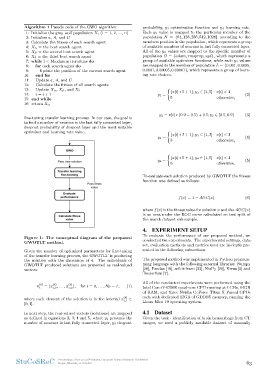
Figure 1: The conceptual diagram of the proposed where f (x) is the fitness value for solution x and the AU C(x)
GWOTLT method. is an area under the ROC curve calculated on test split of
the search dataset sub-sample.
Given the number of optimized parameters for fine-tuning
of the transfer learning process, the GWOTLT is producing 4. EXPERIMENT SETUP
the solution with the dimension of 4. The individuals of
GWOTLT produced solutions are presented as real-valued To evaluate the performance of our proposed method, we
vectors: conducted two experiments. The experimental settings, data-
set, evaluation methods and metrics used are in-depth pre-
xi(t) = (x(i,t0), . . . , x(i,tn) ), for i = 0, . . . , Np − 1 , (1) sented in the following subsections.
where each element of the solution is in the interval xi(,t1) ∈ The proposed method was implemented in Python program-
[0, 1]. ming language with the following external libraries: Numpy
[28], Pandas [18], scikit-learn [22], NiaPy [29], Keras [5] and
In next step, the real-valued vectors (solutions) are mapped Tensorflow [7].
as defined in equations 2, 3, 4 and 5, where y1 presents the
number of neurons in last fully connected layer, y2 dropout All of the conducted experiments were performed using the
Intel Core i7-6700K quad-core CPU running at 4 GHz, 64GB
of RAM, and three Nvidia GeForce Titan X Pascal GPUs
each with dedicated 12GB of GDDR5 memory, running the
Linux Mint 19 operating system.
4.1 Dataset
Given the task - identification of brain hemorrhage from CT
images, we used a publicly available dataset of manually
StuCoSReC Proceedings of the 2019 6th Student Computer Science Research Conference 63
Koper, Slovenia, 10 October
Each y1 value is mapped to the particular member of the
1: Initialize the grey wolf population Xi (i = 1, 2, ..., n) population N = {64, 128, 256, 512, 1024} according to the
2: Initialize a, A, and C members position in the population, which represents a group
3: Calculate the fitness of each search agent of available numbers of neurons in last fully connected layer.
4: Xα = the best search agent All of the y3 values are mapped to the specific member of
5: Xβ = the second best search agent population O = {adam, rmsprop, sgd}, which represents a
6: Xδ = the third best search agent group of available optimizer functions, while each y4 values
7: while i < Maximum iterations do are mapped to the member of population L = {0.001, 0.0005,
8: for each search agent do 0.0001, 0.00005, 0.00001}, which represents a group of learn-
9: Update the position of the current search agent ing rate choices.
10: end for
11: Update a, A, and C y1 = x[i] ∗ 5 + 1 ; y1 ∈ [1, 5] x[i] < 1 (2)
12: Calculate the fitness of all search agents 5 otherwise,
13: Update Xα, Xβ, and Xδ
14: i = i + 1 y2 = x[i] ∗ (0.9 − 0.5) + 0.5; y2 ∈ [0.5, 0.9] (3)
15: end while
16: return Xα x[i] ∗ 3 + 1 ; y3 ∈ [1, 3] x[i] < 1
3 otherwise,
fine-tuning transfer learning process. In our case, the goal is
to find a number of neurons in the last fully connected layer,
dropout probability of dropout layer and the most suitable
optimizer and learning rate value.
y3 = (4)
y4 = x[i] ∗ 5 + 1 ; y4 ∈ [1, 5] x[i] < 1 (5)
5 otherwise,
To evaluate each solution produced by GWOTLT the fitness
function was defined as follows:
f (x) = 1 − AU C(x) (6)
Figure 1: The conceptual diagram of the proposed where f (x) is the fitness value for solution x and the AU C(x)
GWOTLT method. is an area under the ROC curve calculated on test split of
the search dataset sub-sample.
Given the number of optimized parameters for fine-tuning
of the transfer learning process, the GWOTLT is producing 4. EXPERIMENT SETUP
the solution with the dimension of 4. The individuals of
GWOTLT produced solutions are presented as real-valued To evaluate the performance of our proposed method, we
vectors: conducted two experiments. The experimental settings, data-
set, evaluation methods and metrics used are in-depth pre-
xi(t) = (x(i,t0), . . . , x(i,tn) ), for i = 0, . . . , Np − 1 , (1) sented in the following subsections.
where each element of the solution is in the interval xi(,t1) ∈ The proposed method was implemented in Python program-
[0, 1]. ming language with the following external libraries: Numpy
[28], Pandas [18], scikit-learn [22], NiaPy [29], Keras [5] and
In next step, the real-valued vectors (solutions) are mapped Tensorflow [7].
as defined in equations 2, 3, 4 and 5, where y1 presents the
number of neurons in last fully connected layer, y2 dropout All of the conducted experiments were performed using the
Intel Core i7-6700K quad-core CPU running at 4 GHz, 64GB
of RAM, and three Nvidia GeForce Titan X Pascal GPUs
each with dedicated 12GB of GDDR5 memory, running the
Linux Mint 19 operating system.
4.1 Dataset
Given the task - identification of brain hemorrhage from CT
images, we used a publicly available dataset of manually
StuCoSReC Proceedings of the 2019 6th Student Computer Science Research Conference 63
Koper, Slovenia, 10 October